An Introduction to Gaussian Processes

In simple terms, a Gaussian Process (GP) can be thought of as a distribution over functions. It is a supervised machine learning technique for regression (Wikipedia). A key advantage of GPs is that they do not require a parametric model of the data: instead of fitting the coefficients of a chosen formula, they learn directly from the data through a kernel. For an introduction, I recommend the review by Prof. Zoubin Ghahramani, Probabilistic Machine Learning and Artificial Intelligence. Two excellent books are Gaussian Processes for Machine Learning by Carl Edward Rasmussen and Christopher K. I. Williams, and Machine Learning: A Probabilistic Perspective by Kevin Murphy.

The Key Property

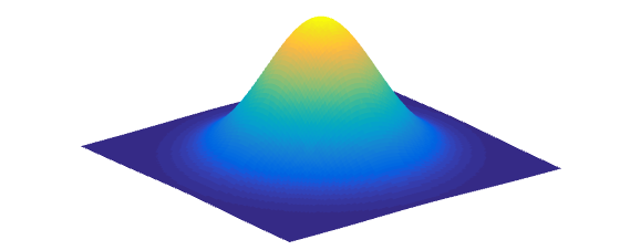
Everything a GP does rests on one property of the multivariate normal distribution: if two variables are jointly Gaussian, then fixing one of them leaves the other Gaussian too. Geometrically, taking a slice through a 2D Gaussian yields another Gaussian, as shown below. Its mean shifts towards the value we fixed, by an amount that depends on how strongly the two variables are correlated, and its variance shrinks, because knowing one variable tells us something about the other.

GP for Regression

In standard Bayesian inference, we choose a parametric model and infer the posterior distribution of its parameters. A GP instead places a prior directly on the function itself, and updates it to a posterior once data are observed. The idea is to treat the unknown function values at the training points and at a new test point, $x_{*}$, as jointly Gaussian. Predicting $f(x_{*})$ then amounts to taking the slice described above: we condition on the values we have observed.

What makes this work is the kernel, which specifies how correlated the function values at two inputs should be. A common choice is the squared-exponential kernel:

\[\kappa(x,\,x') = \sigma^{2}\,\exp\left(-\frac{(x-x')^{2}}{2\ell^{2}}\right)\]

Points close together are strongly correlated, while distant points are almost independent. The length scale, $\ell$, controls how quickly the function can vary horizontally, and the amplitude, $\sigma$, controls how far it can move vertically. Many other kernels exist, each encoding a different belief about the function, such as smoothness or periodicity; Rasmussen and Williams give a thorough overview.

Conditioning on the training data gives the prediction at $x_{*}$ in closed form. With a zero-mean prior and observations corrupted by independent Gaussian noise of variance $\sigma_{n}^{2}$, the predictive mean and variance are

\[\mu_{*} = \mathbf{k}_{*}^{\textrm{T}}\left(\mathbf{K}+\sigma_{n}^{2}\mathbf{I}\right)^{-1}\mathbf{y}, \qquad \Sigma_{*} = k_{**} - \mathbf{k}_{*}^{\textrm{T}}\left(\mathbf{K}+\sigma_{n}^{2}\mathbf{I}\right)^{-1}\mathbf{k}_{*}\]

Here, $\mathbf{K}$ holds the kernel evaluated between all pairs of training points, $\mathbf{k}_{*}$ between the training points and $x_{*}$, and $k_{**}$ at $x_{*}$ itself. The mean is a weighted combination of the observed values, with more weight given to nearby points. The variance starts from the prior uncertainty and is reduced by whatever the data reveal about $x_{*}$. In the noise-free case, we simply set $\sigma_{n}=0$.

Learning the Kernel Parameters

The kernel parameters, $\sigma$ and $\ell$ (and the noise level, if unknown), are usually learned from the data by maximising the marginal likelihood: the probability of the observed data under the GP prior, with the function itself integrated out. This quantity is available in closed form, along with its gradient, so standard optimisers can be used. It also has a built-in preference for simple explanations: a model that is too flexible spreads its probability over too many possible datasets and is penalised automatically. Alternatively, a fully Bayesian approach infers the posterior distribution of the kernel parameters.

Examples

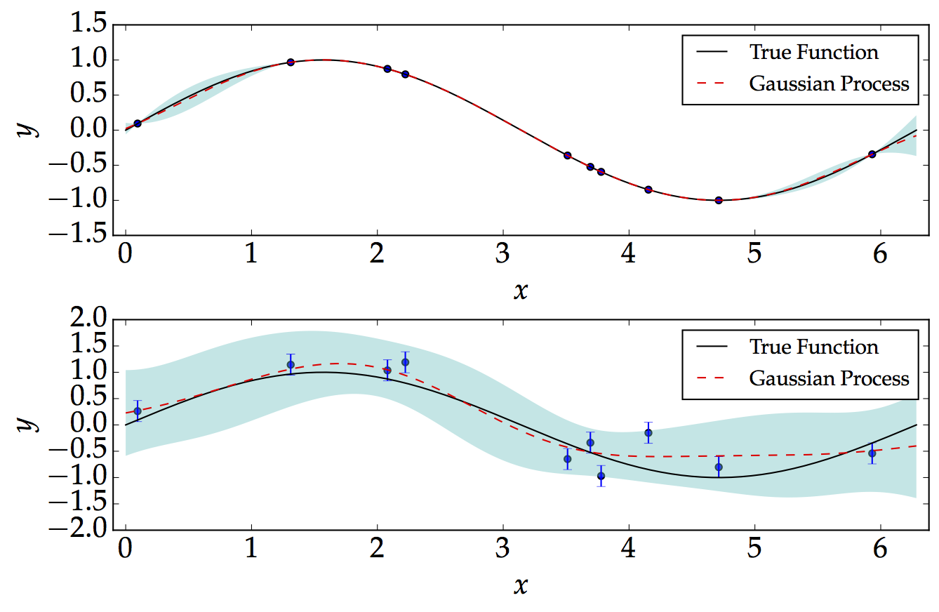
Below are two examples, with both kernel parameters set to 1 for illustration. In the first, the GP learns a sine function on $[0,\,2\pi]$ from noise-free, equally spaced data.

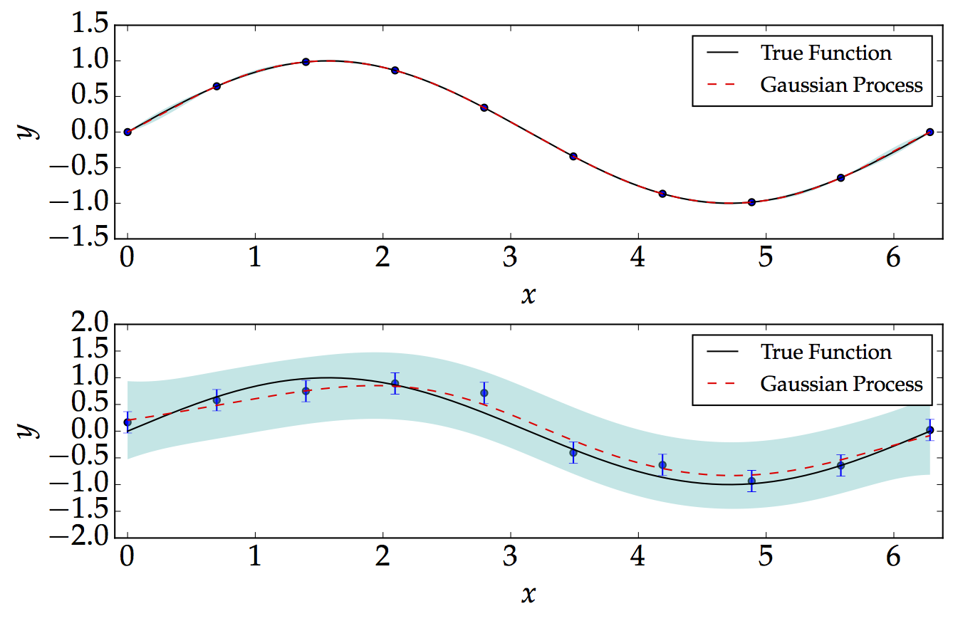
In the second, the data are noisy and unevenly spaced. The key point is that the GP reflects our level of confidence depending on where data are available: predictions are more confident where there are more data, and less confident where there are none.