Parameter Inference with MOPED and Gaussian Processes

In this post, I briefly summarise my first PhD paper, published in MNRAS. A key step in this work is the compression and emulation of the data using MOPED, an algorithm developed by Heavens et al. 2000.

A weak lensing data vector can contain hundreds or thousands of numbers, yet the model it constrains has only a handful of parameters. MOPED compresses a data vector of size $N$ to just $p$ numbers, one per parameter. Each compressed number is a weighted sum of the data, with weights chosen so that it captures as much information as possible about its parameter. The weights are built from the derivatives of the model with respect to each parameter, scaled by the inverse of the noise covariance, and are made mutually orthogonal and normalised. For Gaussian data whose noise covariance does not depend on the parameters, this compression loses no information at the fiducial parameters used to construct it.

The compression also makes the likelihood remarkably simple. Because the weighting vectors are orthogonal and normalised, the compressed numbers are uncorrelated with unit variance, so the log-likelihood reduces to a sum of $p$ squared differences:

\[\log\mathcal{L} = -\frac{1}{2}\sum_{\alpha=1}^{p}\left(y_{\alpha} - \langle y_{\alpha}\rangle\right)^{2} + \textrm{constant}\]

where $y_{\alpha}$ are the compressed data and $\langle y_{\alpha}\rangle$ their theoretical predictions. An MCMC algorithm can then sample the posterior distribution of the model parameters directly from the compressed data.

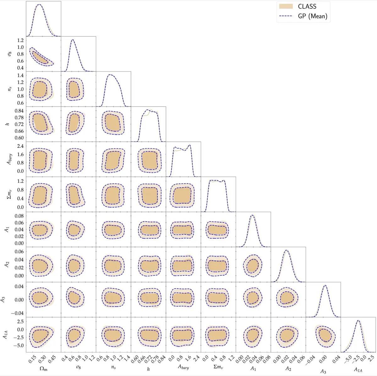
However, computing the theoretical predictions at each step of an MCMC can still be costly when the forward model itself is expensive. We therefore first generate a training set of $N$ Latin Hypercube samples (LHS), compute the MOPED coefficients at these points, and then model them with $p$ separate Gaussian Processes. These serve as surrogates for sampling the posterior distribution of the model parameters, with the result shown in the figure below: the posterior obtained with the full, accurate solver CLASS is shown in tan, and the posterior obtained with the emulator in blue. The contours correspond to the 68% and 95% credible intervals.