An Introduction to Gibbs Sampling

Gibbs sampling is a variant of the Markov Chain Monte Carlo (MCMC) method (Wikipedia). Rather than proposing a move in all parameters at once, it updates one parameter at a time, drawing each from its distribution conditional on the current values of all the others. Cycling through the parameters in this way, over many iterations, produces samples from the full joint posterior.

As with the standard Metropolis-Hastings algorithm, each sample is correlated with its neighbours, so the chain can be thinned by keeping only every n^th value if independent samples are needed. The first part of the chain (the burn-in) is also discarded, as it may not yet represent the target distribution. The main advantage of Gibbs sampling is that there is no proposal distribution to tune: every draw is accepted. The price is that we need to be able to sample from each conditional distribution, which is easy when those conditionals have a standard form.

Example: Bayesian Linear Regression

A straight-line fit illustrates the method well. Suppose we have data points $(x_{i},\,y_{i})$ generated from

where $\epsilon$ is Gaussian noise with known standard deviation. We want the full posterior distribution of the intercept, $\theta_{0}$, and the gradient, $\theta_{1}$, and place an independent Gaussian prior on each.

This choice makes Gibbs sampling particularly convenient. With a Gaussian likelihood and Gaussian priors, the log-posterior is a quadratic function of each parameter when the other is held fixed. Completing the square then shows that each conditional distribution is itself Gaussian. For example, the distribution of $\theta_{0}$ given $\theta_{1}$ has a mean that balances what the data imply for the intercept (after subtracting the current gradient term) against the prior mean, weighted by their respective precisions, and a variance that shrinks as more data are added. The same holds for $\theta_{1}$ given $\theta_{0}$. Both conditionals are simple enough to write in a few lines of code, which is exactly what the functions below do.

Python Code

We now have everything we need to write the Python code. The simulated data are available on GitHub. We first define the linear function and the true parameters: 2.0 for the gradient, $\theta_{1}$, and 0.5 for the y-intercept, $\theta_{0}$. In the code below, m and c denote the gradient and the y-intercept. We also specify the fraction of the chain to be treated as burn-in.

def linear(params):
	return params[0]*x + params[1]

# True Parameters
grad  = 2.0
yint  = 0.5

# Fraction considered as burn-in
frac  = 0.2

# Load the data 
data  = np.loadtxt('data_gibbs.txt')
x     = data[:,0]; xmin = min(x); xmax = max(x)
y     = data[:,1]
sigma = data[:,2]

The next step is to scale the data by their uncertainties, so that each point is weighted according to its precision. We also define the hyper-parameters of the Gaussian priors and the functions used to sample $m$ and $c$, respectively. A further function is used to find the best-fit parameters by optimisation, which then serve as the starting point for the Gibbs sampler.

# Create Design Matrices
Dm = x/sigma
Dc = 1.0/sigma
b  = y/sigma

# Define Priors (Gaussian Priors)
mu_m = 2.0; mu_c = 1.0
si_m = 2.0; si_c = 2.0

# Define Functions for Sampling
def sample_grad(m, c):
	var  = 1.0/(np.dot(Dm.T, Dm) + 1.0/si_m**2)
	mean = var*(np.dot(b.T, Dm) + (mu_m/si_m**2) - c * np.dot(Dc.T, Dm))
	return np.random.normal(mean, np.sqrt(var))

def sample_yint(m, c):
	var  = 1.0/(np.dot(Dc.T, Dc) + 1.0/si_c**2)
	mean = var*(np.dot(b.T, Dc) + (mu_c/si_c**2) - m * np.dot(Dc.T, Dm))	
	return np.random.normal(mean, np.sqrt(var))

# Define the log-likelihood for optimisation
def loglikelihood(theta, data, Sigma):
  theta0, theta1 = theta 
  model     = linear(theta)
  chiSquare = LA.norm((model - data)/Sigma)**2
  loglike   = -0.5 * (chiSquare) 
  return loglike

# Use, for example, Powell method for optimisation
chi_square = lambda *args: -2*loglikelihood(*args)
result     = op.minimize(chi_square, [1.0, 1.0], args=(y, sigma), method = 'Powell', tol = 1E-5)
theta_op   = np.array(result["x"])

m = theta_op[0]
c = theta_op[1]

We are now ready to run the sampler. We fix the number of iterations at 200 000 and discard the first 20% of the chain.

iters = 2E5
trace = np.zeros(shape = (int(iters), 2))

def gibbs(m, c):

	for i in range(int(iters)):
		m = sample_grad(m, c)
		c = sample_yint(m, c)
		trace[i,:] = np.array([m, c])

	return trace

samples = gibbs(m,c)
samples = samples[int(frac*iters):] # Reject first 20 % of the chains

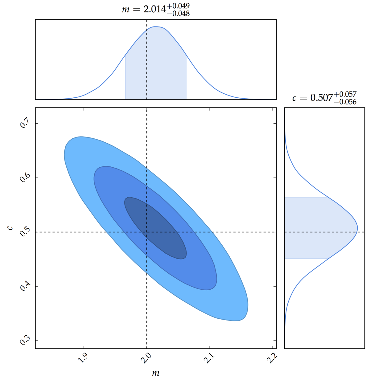
Finally, we obtain the 2D posterior distribution of the parameters.