Sampling from Any Distribution

Drawing random samples from an arbitrary distribution is a common task, yet practical guidance on it is surprisingly scattered. Here, we present three methods for generating random numbers from a distribution: built-in functions in scipy, acceptance-rejection sampling, and an interpolation method. The distribution we use is

\begin{align} \mathcal{P}\left(x\right) = \dfrac{k\,x^3}{e^{2x} - 0.1} \end{align}

where $k$ is the normalisation constant. Below, PDF stands for the probability density function and CDF for the cumulative distribution function. The shape of this distribution resembles that of a black-body spectrum. It is used here purely to illustrate sampling; we do not discuss the physics of black-body radiation in this post.

Using Scipy

The class rv_continuous in scipy.stats is straightforward to use. We simply define either the PDF or the CDF, using _pdf or _cdf respectively, as shown below. We first define the PDF and then a function to normalise it; note that the PDF defined in the class must be normalised.

x = np.linspace(0.0, 10.0, 1E4)

def p(x):
	return (x**3)/(np.exp(2.0 * x) - 0.1)

# Define function to normalise the PDF
def normalisation(x):
	return simps(p(x), x)

# Define the distribution using rv_continuous
class blackbody(ss.rv_continuous): 
    def _pdf(self, x, const):
        return (1.0/const) * p(x)

We can now use these functions to compute the PDF and the CDF, and to generate samples from the underlying distribution. We first instantiate the distribution with lower and upper limits given by a and b, respectively. If these are not specified, the support defaults to $-\infty$ to $+\infty$.

blackbody_distribution = blackbody(name="blackbody_distribution", a=0.0)

# Find the normalisation constant first
norm_constant = normalisation(x)

# create pdf, cdf, random samples
pdf = blackbody_distribution.pdf(x = x, const = norm_constant)
cdf = blackbody_distribution.cdf(x = x, const = norm_constant)
samples = blackbody_distribution.rvs(const = norm_constant, size = 1E4)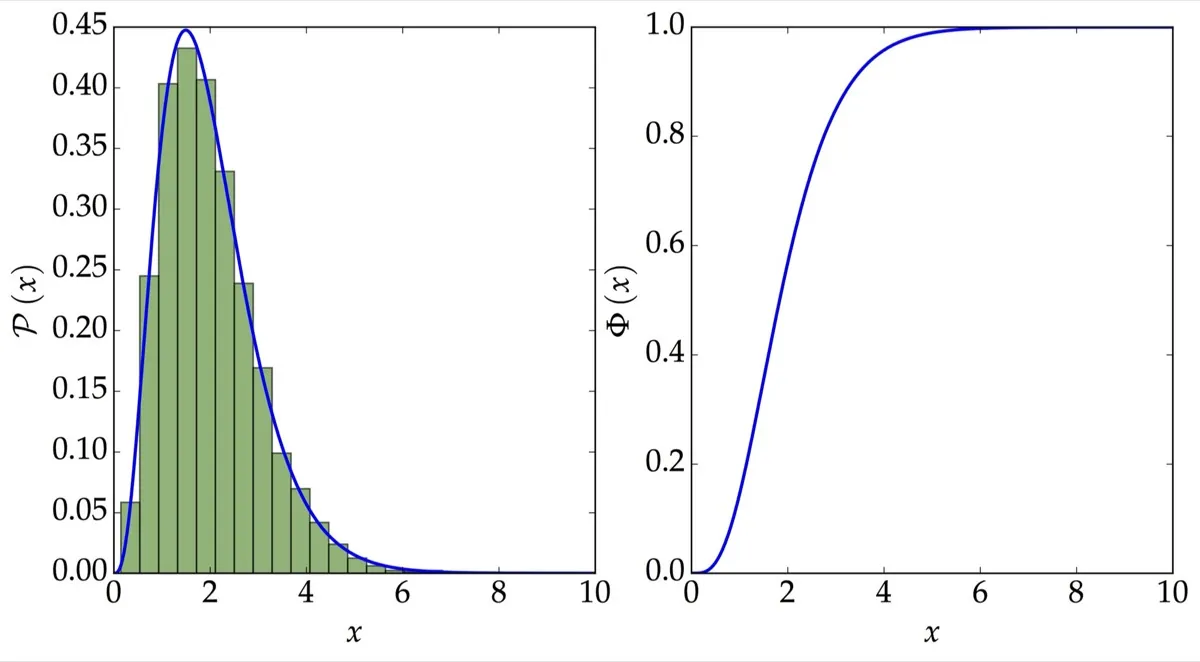

The plot above shows the PDF, the CDF and 10 000 random samples drawn from the distribution. rv_continuous is particularly useful when more than just samples are needed: once it is defined, other properties such as the mean and standard deviation are readily available (see the documentation for further details).

Acceptance-Rejection Sampling

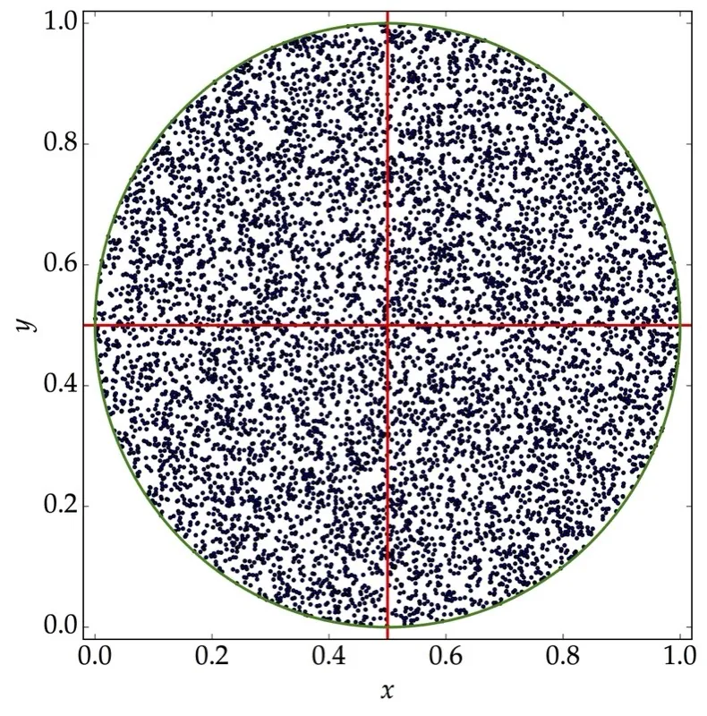
Imagine a square board of side $l$, with a circle of radius $0.5l$ at its centre, that is, at $\left(0.5l,0.5l\right)$ in Cartesian coordinates. Suppose we throw darts randomly at the board $N$ times. If $n$ darts land inside the circle, the probability of hitting the circle is simply $\frac{n}{N}$, which is approximately the ratio of the area of the circle to that of the board. This idea gives a rough estimate of $\pi$:

\begin{align} \pi \approx 4 \times \frac{n}{N} \end{align}

As $N$ increases, the estimate of $\pi$ becomes more accurate. This is the idea behind Monte Carlo sampling. In the same spirit, another way to sample from a normalised distribution is acceptance-rejection sampling, sometimes called Lahiri's sampling method. Its advantage is that the CDF is not needed. One drawback, however, is that samples may be rejected very often, so obtaining a desired number $N$ of random numbers can take a long time. We have not implemented this method in this post. In short,

suppose $X$ is a scalar random variable taking values in the interval $\left[a, b\right]$ according to the continuous probability density function $f\left(x\right)$. Let $M$ be an upper bound for $f$ on $\left[a, b\right]$, $M$ assumed finite. Choose $x$ uniformly in $\left[a, b\right]$. Then choose $u$ uniformly in $\left[0, M\right]$. If $u\leq f\left(x\right)$, we select $x$. Otherwise we reject $x$ and start over.

Interpolation Method

What if neither of these methods works, but we do have the PDF? In that case, we proceed as follows:

1. Find the CDF using np.cumsum
2. Generate a random number from a uniform distribution, $\mathcal{U}\left[0,1\right]$
3. Use interp1d from scipy.interpolate to estimate the random number.

# Our Own pdf, cdf and samples
own_pdf = p(x)/norm_constant
own_cdf = np.cumsum(own_pdf); own_cdf /= max(own_cdf)

# Define a function to return N samples
def genSamples(N):
	u = np.random.uniform(0, 1, int(N))
	func_interp = interp1d(own_cdf, x)
	samples = func_interp(u)
	return samples

own_samples = genSamples(1E4)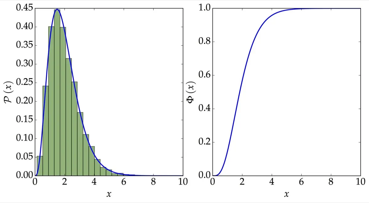

This gives 10 000 random samples drawn using the CDF, and the result closely matches the one obtained with rv_continuous.