Linear Regression with Maximum Likelihood
Maximum likelihood fitting, applied to an A-Level physics experiment.
A common problem in statistics is learning the functional relationship between independent variables and a dependent variable. For example, we may want to know how house prices vary with the area of the land, the total size of the house and other criteria. Here, the house price is the dependent variable, often called the response variable, while the land area and total size of the house are the independent variables, also known as attribute variables.
We begin with linear modelling: given a set of attributes, we want to infer a linear relationship between the attributes and the response. The function we want to fit is typically governed by a set of parameters, say $\theta_{i}$. Before going further, however, it is worth distinguishing between linear and non-linear models.
The equation \begin{align} y=\theta_{0} + \theta_{1}x + \theta_{2}x^2 \end{align} is a linear model because it is linear in the parameters $\theta_{i}$. In contrast, the model \begin{align} y=\textrm{sin}\left(\omega x + \phi\right) \end{align} is a non-linear model, since it is non-linear in the parameters $\left(\omega,\,\phi\right)$.
Maximum Likelihood Method
Suppose we want to fit a straight line, $f(x) = \theta_{0} + \theta_{1}x$, to some observed data points $(x_{i},\,y_{i})$, each with a known Gaussian measurement error, $\sigma_{i}$. The likelihood measures how probable the observed data are for a given choice of parameters. For Gaussian errors, maximising it amounts to finding the line that minimises the familiar weighted sum of squared residuals, often called $\chi^{2}$, in which each point counts in proportion to its precision: points with small error bars pull the line harder than points with large ones.
For a linear model, this problem has an exact solution. Writing the scaled data as a vector $\mathbf{b}$ (each $y_{i}$ divided by its error) and the model as a design matrix $\mathbf{D}$ (with one column per parameter, likewise scaled), setting the gradient of the likelihood to zero gives
\[\boldsymbol{\theta}_{\textrm{MLE}} = \left(\mathbf{D}^{\textrm{T}}\mathbf{D}\right)^{-1}\mathbf{D}^{\textrm{T}}\mathbf{b}\]The matrix $\mathbf{C} = \left(\mathbf{D}^{\textrm{T}}\mathbf{D}\right)^{-1}$ is just as useful: it is the covariance matrix of the fitted parameters. Its diagonal elements are the variances of the parameters, so their square roots give the error bars, and its off-diagonal elements tell us how the parameters are correlated.
Example - A Physics Problem
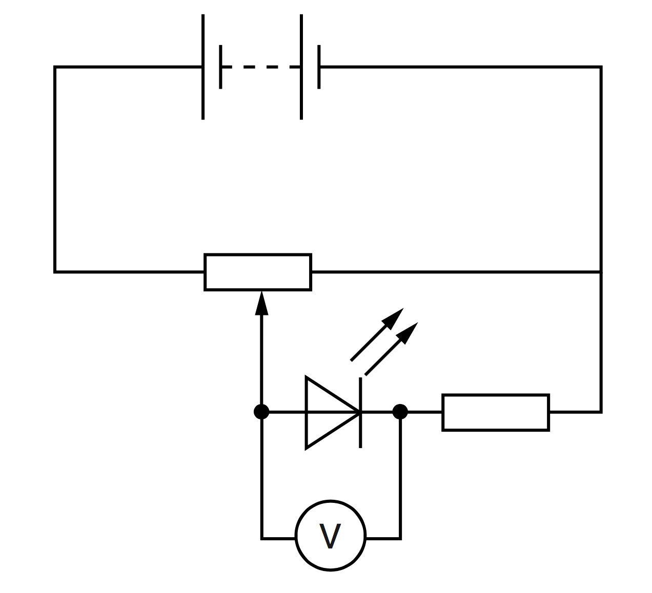
We now apply this method to a physics problem (Physics 9702, November 2016, Paper 52). A student is investigating the characteristics of different light-emitting diodes (LEDs). Each LED needs a minimum potential difference across it to emit light. The circuit is set up as shown on the left.
The potentiometer is adjusted until the LED just emits light. The potential difference $V$ across the LED is measured. The experiment is repeated for LEDs that emit light of different wavelength $\lambda$. It is suggested that $V$ and $\lambda$ are related by the equation \begin{align} V=p\lambda^{q} \end{align} where $p$ and $q$ are constants. Taking logarithms turns this into a straight line: if we plot $\textrm{lg }V$ against $\textrm{lg }\lambda$, the gradient is $q$ and the $y$-intercept is $\textrm{lg }p$, so the method above applies directly.
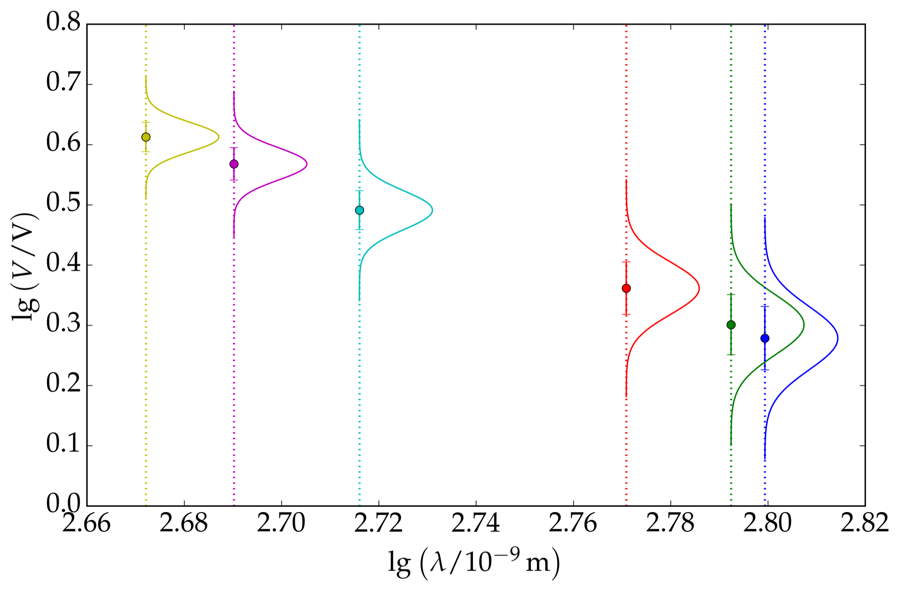
The values of $V$ and $\lambda$ are given in the table below, together with $\textrm{lg }\lambda$ and $\textrm{lg }V$ and its associated error, which is the fractional error in $V$. We calculate $\textrm{lg }\lambda$ and $\textrm{lg }V$ to two decimal places, and assume that each data point is Gaussian distributed with mean $\mu=\textrm{lg }V$ and standard deviation $\sigma = \sigma_{\textrm{lg }V}$, as illustrated on the right. Plotting $\textrm{lg }V$ against $\textrm{lg }\lambda$, we find a gradient of $-2.60$ and a $y$-intercept of $7.56$.
| $\lambda/10^{-9}$ m | $V/\,\textrm{V}$ | $\textrm{lg}\left(\lambda/10^{-9}\,\textrm{m}\right)$ | $\textrm{lg}\left(V/\,\textrm{V}\right)$ |
|---|---|---|---|
| 630 | $1.9\pm0.1$ | 2.80 | $ 0.28\pm0.05$ |
| 620 | $2.0\pm0.1$ | 2.79 | $0.30\pm0.05$ |
| 590 | $2.3\pm0.1$ | 2.77 | $0.36\pm0.04$ |
| 520 | $3.1\pm0.1$ | 2.72 | $0.49\pm0.03$ |
| 490 | $3.7\pm0.1$ | 2.69 | $0.57\pm0.03$ |
| 470 | $4.1\pm0.1$ | 2.67 | $0.61\pm0.02$ |
The square roots of the diagonal of the covariance matrix give the uncertainties on the two parameters, so that $q=-2.60\pm0.31$ and $\textrm{lg }p = 7.56\pm0.82$. The off-diagonal element, $-0.258$, is negative, which already tells us that the two estimates are anti-correlated.
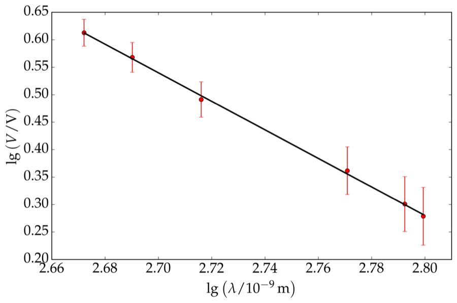
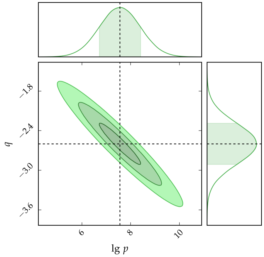
In summary, the estimates of $p$ and $q$ are $3.61\times10^{7}$ and $-2.60$, respectively. Because the off-diagonal elements of the covariance matrix are negative, the parameters are negatively correlated: an increase in one corresponds to a decrease in the other, as the tilted contours in the right-hand figure show. The joint distribution of $\left(\textrm{lg }p,\,q\right)$ is Gaussian, since we are working with a linear model. Finally, the values of $p$ and $q$ can be used to estimate the minimum potential difference required for a different diode, for example, one emitting at a wavelength of $950$ nm.
Summary and Conclusion
In this post, we have covered one method of inferring parameters, the Maximum Likelihood Estimator, and illustrated it with an example. The method provides good estimates of the parameters and their associated errors, and the covariance matrix also reveals the correlations between the parameters.
If we had prior information on the parameters, we would turn to Bayesian statistics. The approach is similar, except that each parameter would have a prior probability distribution, and instead of the MLE we would obtain the MAP, or Maximum a Posteriori, estimates of the parameters. With uniform priors, the MAP and MLE coincide.