Bayesian School 2016
Highlights from the 2016 Bayesian School: KL divergence and BHMs.
The 2016 Bayesian School was held at Stellenbosch University from 21 to 25 November. The school focused on three main topics: Introductory Bayesian Methods, Monte Carlo Methods and Advanced Bayesian Methods, the last of which was taught by Prof. Alan Heavens from Imperial College.
Beyond the lectures, another interesting part of the school was the "Research Hacks", which allowed participants to meet in small groups, ask questions, exchange ideas and initiate collaborations. The hacks largely served these purposes and also led to the publication of three papers (see arXiv:1704.03472, arXiv:1704.03467 and arXiv:1704.07830).
I learned a great deal from Prof. Heavens' lectures and attempted some of the problems he set during the school. There were also several other interesting lectures on Bayesian methods. Below, I discuss two topics: the KL divergence and Bayesian Hierarchical Modelling.
Kullback-Leibler (KL) Divergence
In a Bayesian analysis, a prior distribution, $\pi(\boldsymbol{\theta})$, is updated by the data into a posterior distribution, $q(\boldsymbol{\theta})$. A natural question is how much we have learned from the experiment. The Kullback-Leibler (KL) divergence answers it:
\[\textrm{D}_{\textrm{KL}}(q\,\Vert\,\pi) = \int q\,\log\left(\frac{q}{\pi}\right)d\boldsymbol{\theta}\]Also known as the relative entropy, it is measured in bits when logarithms are taken to base 2, and in nats when they are taken to base $e$. For two Gaussians, it has a simple closed form, and two effects stand out. The information gain grows as the posterior becomes narrower than the prior, and it grows further when the posterior mean has moved away from the prior mean: we learn the most from an experiment that both tightens and shifts our beliefs.
One of the exercises made this concrete:
We have an experiment where a single datum $x$ is assumed to be drawn from a Gaussian likelihood of mean $\mu$ and variance $\sigma^{2}$. Compute the KL divergence between an assumed Gaussian prior on $\mu$ (with mean zero and variance $\Sigma$) and the posterior.
Working through the algebra, the information gain depends on how wide the prior is compared with the measurement error, and on how surprising the datum is. The interesting limit is a prior of zero width, a Dirac delta, which amounts to claiming we already know $\mu$ exactly. The information gain is then zero: no experiment can teach us anything. In my view, this example highlights the importance of stating priors honestly, which in turn makes the case for the Bayesian formalism.
Bayesian Hierarchical Modelling
This topic helped me answer a question I had long wondered about: how should we perform parameter inference when both the dependent and independent variables have error bars? The idea behind Bayesian Hierarchical Modelling (BHM) is to split the problem into steps, so that the full model consists of a series of linked sub-models, with uncertainties propagated from one to the next.
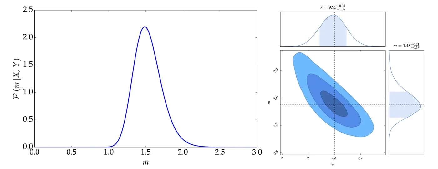
Consider a simple example: fitting a straight line, $y=mx$, to a single measured point, $(X,\,Y)$, where both coordinates have errors. How do we infer $m$?
The trick is to introduce the true, unobserved values, $x$ and $y$, as latent variables. The model then has three layers: the slope, $m$, determines the true $y$ from the true $x$; the measurements $X$ and $Y$ scatter around the true values according to their errors; and since we do not care about the true values themselves, we integrate them out at the end. With Gaussian errors of unit variance on both coordinates and uniform priors, the integral can be done analytically, giving the posterior distribution of the slope:
\[\mathcal{P}(m\,|\,X,\,Y) \propto \frac{1}{\sqrt{1+m^{2}}}\,\exp\left[-\frac{1}{2}\left(\frac{Y-mX}{\sqrt{1+m^{2}}}\right)^{2}\right]\]The factor $\sqrt{1+m^{2}}$ is where the error in $X$ shows up: a steeper line magnifies any uncertainty in $x$ into a larger uncertainty in $y$. Alternatively, rather than integrating out $x$, we can keep it and sample the joint posterior of $x$ and $m$ directly, for example with Gibbs sampling.
Consider the case $X=10$ and $Y=15$. The left panel of the figure below shows the posterior distribution of $m$ from the formula above, and the right panel shows the joint posterior distribution of $x$ and $m$ obtained with Gibbs sampling.