Bayesian Evidence: The Gaussian Linear Model

Following our recent post on Bayesian Model Selection, we now illustrate it with a simple example: calculating the Bayesian evidence for the Gaussian Linear Model. Consider the figure below.

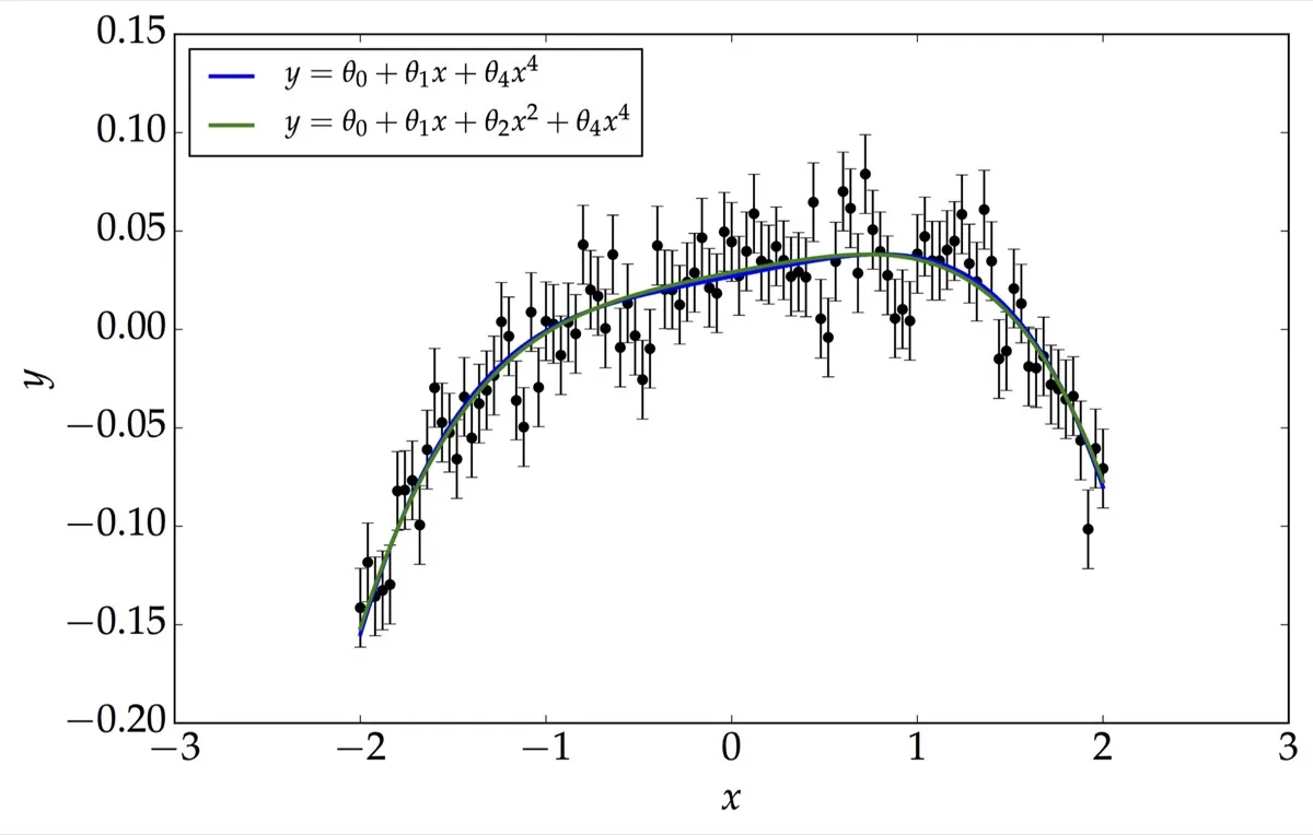
Our data are dominated by noise, $\mathbf{n}\sim\mathcal{N}(0,\,0.02)$. We consider two models, $\mathcal{M}_{1}$ and $\mathcal{M}_{2}$:

\[\mathcal{M}_{1}:\; y=\theta_{0}+\theta_{1}x+\theta_{2}x^{2}+\theta_{4}x^{4}\] \[\mathcal{M}_{2}:\; y=\theta_{0}+\theta_{1}x+\theta_{4}x^{4}\]

It is very difficult to choose the better model simply by looking at the fits. Both were obtained by Maximum a Posteriori (MAP) estimation, with a Gaussian prior of mean 0 and variance 1 on each parameter. Setting $\theta_{2}$ to zero reduces $\mathcal{M}_{1}$ to $\mathcal{M}_{2}$, a common situation in fitting problems. If we naively compare the models by their $\chi^{2}$, the model with more parameters will always win, since an extra parameter can only improve the fit. This is overfitting, and we should be wary of it.

The Bayesian evidence avoids this trap, and for this problem it can be computed exactly. Because the model is linear in its parameters, and both the likelihood and the prior are Gaussian, the integrand of the evidence is itself a Gaussian in the parameters. Two standard tools, completing the square and the multi-dimensional Gaussian integral, then give the evidence in closed form, with no sampling required. The result has a clear interpretation: it rewards the best fit achievable, and penalises the model by the ratio of the volume of parameter space allowed after seeing the data to the volume allowed by the prior. Each extra parameter that the data do not really need pays this penalty.

For our data, the log-evidences of $\mathcal{M}_{1}$ and $\mathcal{M}_{2}$ are 238.458 and 243.338, respectively. The log-Bayes factor, which is simply their difference, is therefore 4.88 in favour of $\mathcal{M}_{2}$: moderate evidence for the simpler model on the Jeffreys scale from our previous post, and close to the threshold for strong evidence. The extra $x^{2}$ term is not justified by the data.

SDDR - Savage-Dickey Density Ratio

In most problems, the evidence is a multi-dimensional integral with no closed form, and computing it is expensive. When the models are nested, as here, there is a useful shortcut: the Savage-Dickey Density Ratio (SDDR). Suppose the extended model, $\mathcal{M}_{1}$, has parameters $(\boldsymbol{\psi},\,\boldsymbol{\phi})$ and reduces to the simpler model, $\mathcal{M}_{0}$, when $\boldsymbol{\phi}=\boldsymbol{\phi}_{0}$. If the priors on $\boldsymbol{\psi}$ and $\boldsymbol{\phi}$ are independent, as is common, the Bayes factor is

\[B_{01} = \left.\frac{\mathcal{P}(\boldsymbol{\phi}\,|\,\mathcal{D},\,\mathcal{M}_{1})}{\mathcal{P}(\boldsymbol{\phi}\,|\,\mathcal{M}_{1})}\right|_{\boldsymbol{\phi}=\boldsymbol{\phi}_{0}}\]

In words, the SDDR is the ratio of the marginal posterior to the prior of the extra parameters, evaluated at the values that recover the simpler model. If the data pile posterior probability onto $\boldsymbol{\phi}_{0}$, the simpler model is favoured; if they move it away, the extra parameters are warranted. Both quantities can be read off an ordinary MCMC run of the extended model, so the Bayes factor comes almost for free, without computing either evidence.