An Iterative Method for Likelihood Emulation
Likelihood emulation with Gaussian Processes and Bayesian optimisation.
The paper 'Cosmological parameter estimation via iterative emulation of likelihoods' was recently posted on arXiv. The idea is to use a Gaussian Process to emulate the log-likelihood and to progressively augment the training set using Bayesian Optimisation. In this post, I illustrate the technique with a simple straight-line fitting example, which should be easy to follow.
Analytical Posterior
We begin by drawing 50 points uniformly at random from $x\in[0, 1]$ and compute $\mathbf{y}$, which is given by $$ \mathbf{y} = \theta\mathbf{x} + \boldsymbol{\epsilon} $$
We fix $\theta = 1$, add Gaussian noise with a standard deviation of 0.04, and place a Gaussian prior on $\theta$ with mean 1 and variance 1. Because the model is linear and both the noise and the prior are Gaussian, the posterior distribution of $\theta$ is also Gaussian and can be written down exactly. This gives us a reference answer against which to check the emulator.
Gaussian Process and Bayesian Optimisation
A Gaussian Process (GP) is a distribution over functions (see this post for an introduction). Trained on a handful of evaluations of the log-likelihood, it predicts the log-likelihood everywhere else, together with an uncertainty that is small near the training points and large far from them.
Bayesian Optimisation is a strategy for finding the optimum of a function that is expensive to evaluate. A typical example arises in cosmology, where a series of integrations and other costly calculations (for example, to account for systematics) must be performed before the log-likelihood can be computed. Rather than evaluating the function on a dense grid, we use the GP to decide where the next evaluation will be most useful.
Acquisition Functions
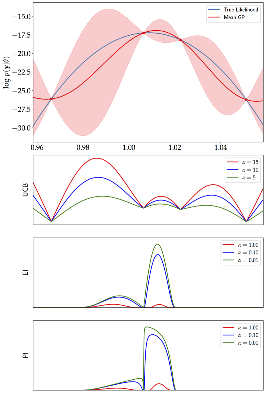
That decision is made by an acquisition function, which scores every candidate point using the GP's prediction and uncertainty. Several choices exist. The probability of improvement picks the point most likely to beat the best value found so far. The expected improvement also accounts for how large that improvement is likely to be. The upper confidence bound (UCB) simply adds a multiple of the uncertainty to the prediction:
\[\textrm{UCB}(\theta) = \mu(\theta) + \alpha\,\sigma(\theta)\]The parameter $\alpha$, set by the user, controls the trade-off between exploitation (sampling where the predicted log-likelihood is high) and exploration (sampling where the GP is most uncertain).
Our Implementation
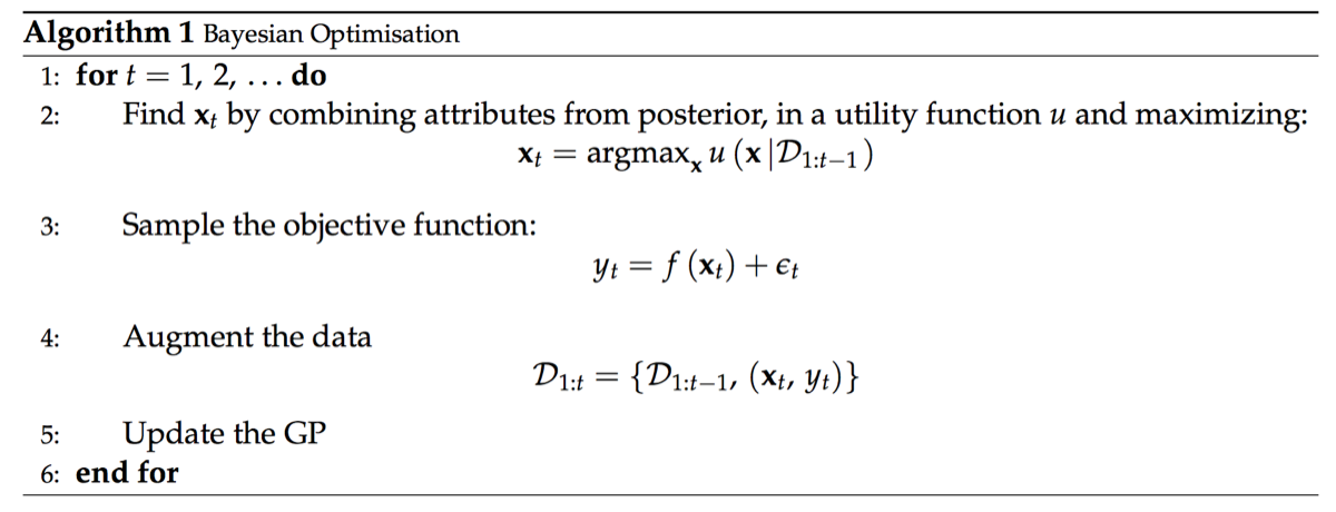
We start with just four training points (generated using Latin Hypercube Sampling, LHS), shown in the first four rows of the table below. We then use the Upper Confidence Bound (UCB) acquisition function (with $\alpha=15$) to iteratively add two points (the last two rows, in red) to the Gaussian Process model. See the algorithm below for further details.
| $\theta$ | $\textrm{log } L$ |
|---|---|
| 0.9662 | -26.1204 |
| 1.0064 | -17.2318 |
| 1.0223 | -18.1605 |
| 1.0511 | -26.2248 |
| 0.9860 | -19.7343 |
| 1.0369 | -21.2069 |
Results and Conclusions
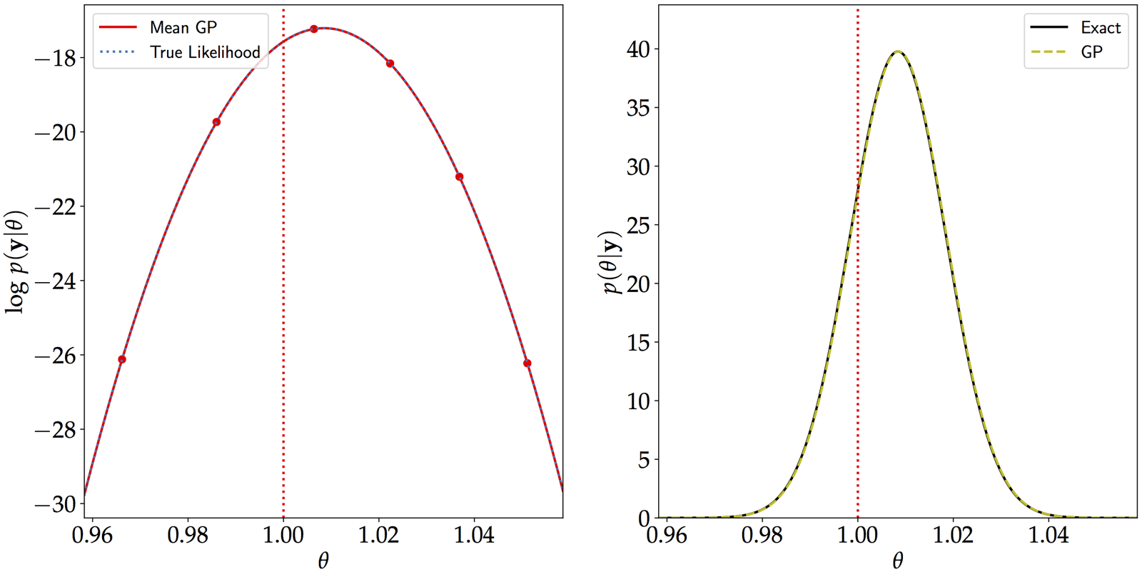
In this setup, we can reconstruct the log-likelihood almost perfectly after augmenting the data set in just two iterations. As the right-hand panel below shows, the resulting posterior distribution of $\theta$ is identical to the exact, analytically derived one. The vertical dashed line marks the value $\theta=1$ used to generate the data.
In high dimensions, however, the volume of the parameter space grows, and reconstructing a function perfectly (if that is the main objective) becomes difficult. Moreover, the acquisition functions themselves have multiple local optima (as seen in the figure at the top), and the choice of acquisition function is an interesting research question in its own right. Acquisition functions can be greedy, favouring exploitation over exploration, so the choice of $\alpha$ also matters.
References